On 23 June 2020, I gave a keynote talk in SWAT 2020. You can watch the talk on YouTube, but for the benefit of those who prefer text to videos, here is the full transcript of the talk, together with the key parts of the presentation slides and some links to the key references. You can find the abstract of the talk in the conference proceedings.

Hello everyone, and welcome! I am Jukka Suomela from Aalto University, and today I’ll talk about the theoretical foundations of the modern world.

If we look at the world around us, we see that it heavily relies on world-wide communication networks and large-scale distributed systems. Just think about all the network infrastructure you are using right now to watch this talk. Systems like mobile phone networks and the global Internet are truly amazing achievements of engineering, but what’s the theoretical foundation for our understanding of such systems? One of the fields that studies such foundational questions is the theory of distributed computing.

In the theory of distributed computing, the key question is this: What can be computed efficiently in a large computer network?

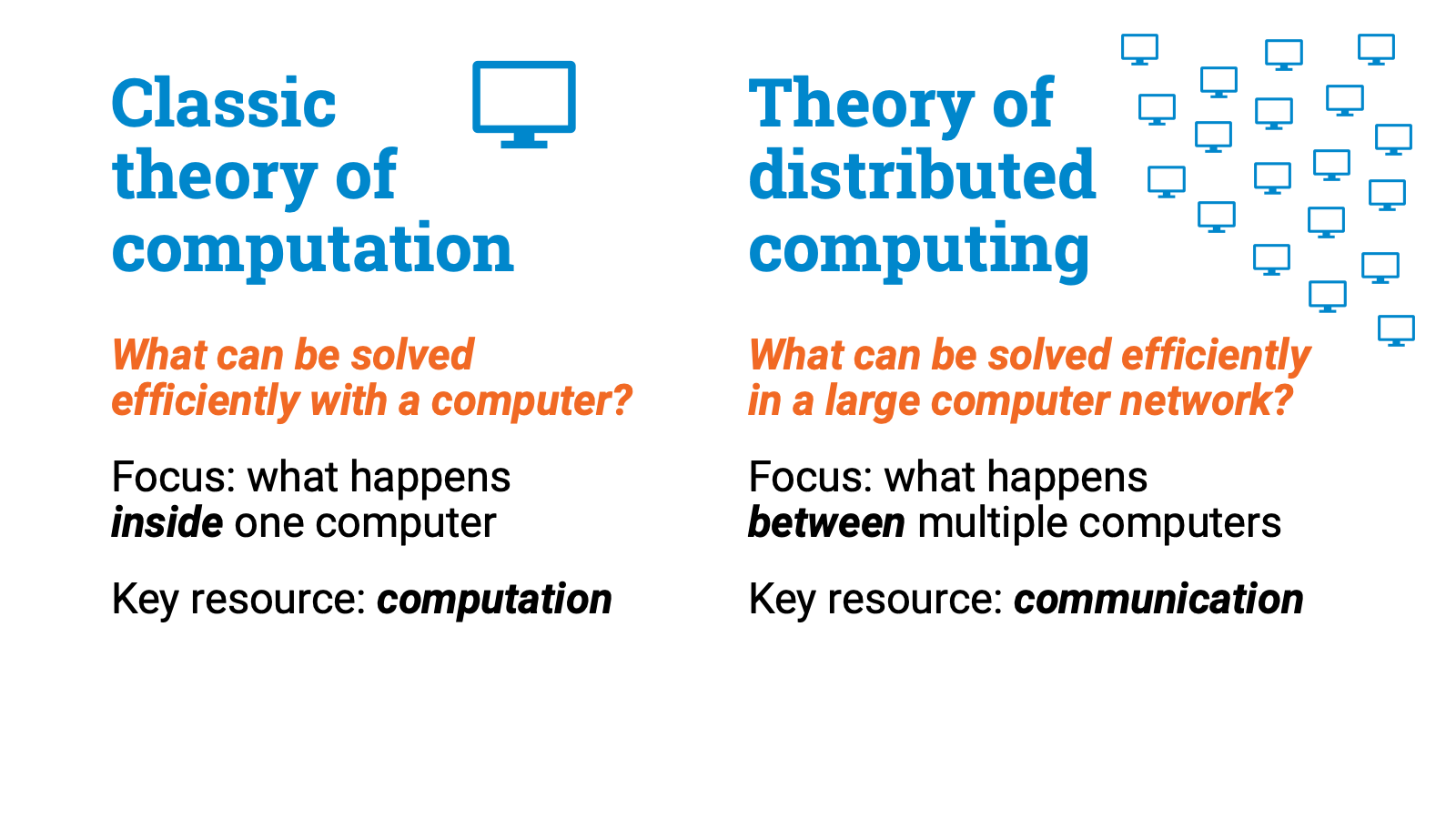
It’s useful to contrast this with the classic theory of computation, where the key question is what can be solved efficiently with a single computer.

While the classic theory of computing is interested in what happens inside one computer, in distributed computing we are interested in what happens between multiple computers.

The key resource is not computation but communication.

Of course you can measure communication from many different perspectives, but perhaps the most fundamental limitation is the latency of communication.

Remember that there is no way to exceed the speed of light in communication. No matter how much or how little data you send from one computer to another, it will take at least some fixed amount of time, depending on the distance.

You can always buy more bandwidth between two computers. You can install more and more parallel fiber-optic links between two data centers. But you can’t reduce latency beyond a certain point. You can’t transmit data faster than light. Every communication step takes some amount of time.

And, if you look at real-world computer networks in practice, you can see that communication steps are usually very expensive in comparison with computation steps. Get one bit of data from a computer next door, and you’ll usually spend several milliseconds. Even if you just try to get one bit of data from another computer sitting in your local network, you’ll still have to wait for maybe half a millisecond.

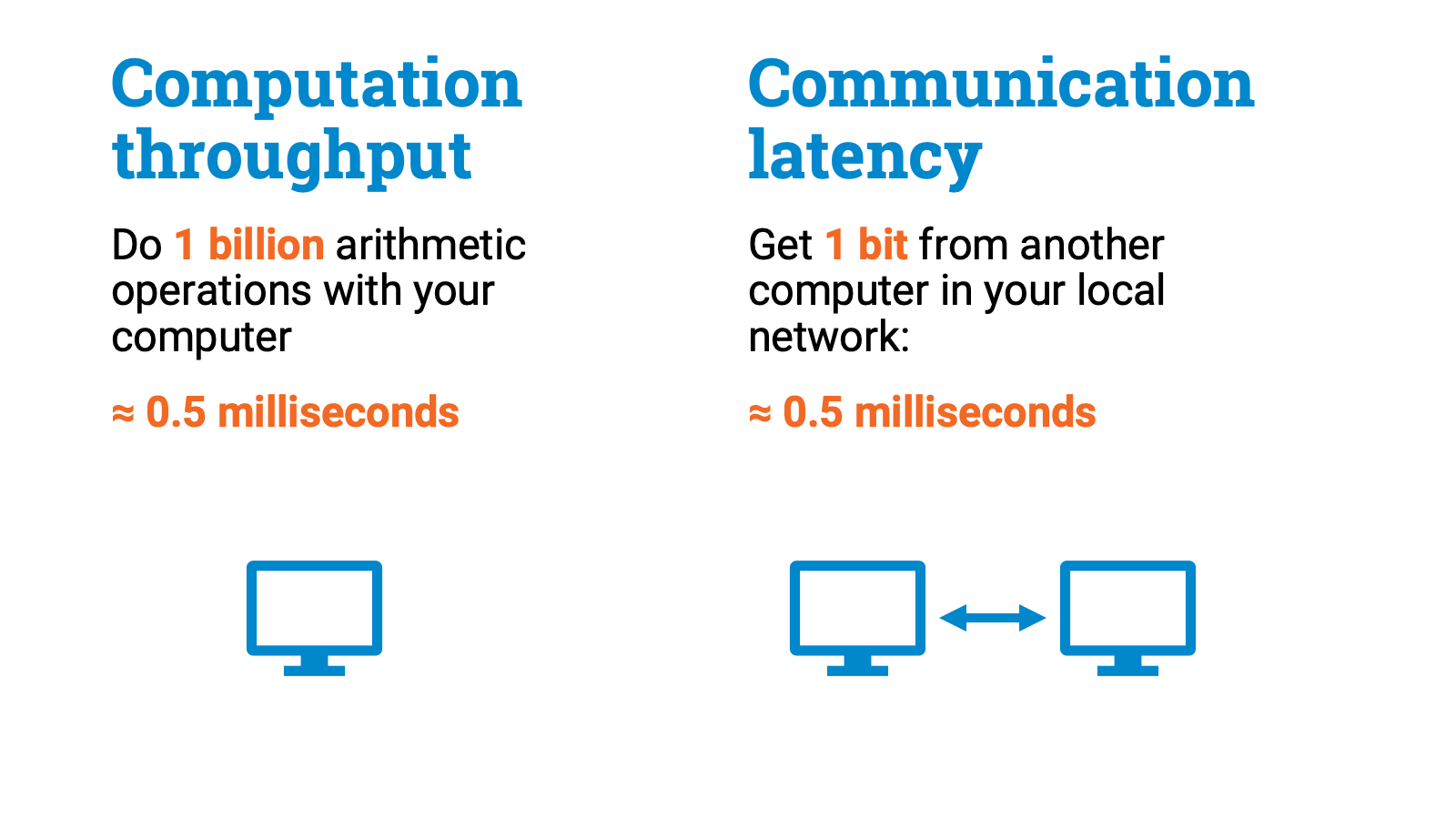
It doesn’t sound like much, until you check how many arithmetic operations your computer could do in half a millisecond. And even for your old desktop computer the answer can be easily one billion!

So to a first approximation, computation is basically free, and all that matters is the number of communication steps that we need.

So an efficient algorithm for computer networks is an algorithm that takes as few communication steps as possible. And this is one of the key questions that we want to understand in the theory of distributed computing:

• what computational problems can be solved in a small number of communication rounds, and
• what computational problems necessarily require a large number of communication rounds?

This idea is formalized in a model of computing called the LOCAL model. This model was introduced in the late 1980s by Linial, and it’s delightfully simple and elegant.

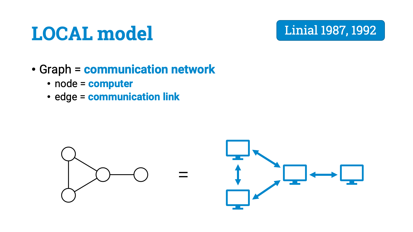
We’ve got some graph, and the graph represents our computer network. Each node is a computer. Each edge is a communication link.

All nodes run the same algorithm. The nodes have unique identifiers, and maybe some other local inputs, but other than that they are identical.

Computation proceeds in synchronous rounds. In each round, each node sends a message to each neighbor, it receives a message from each neighbor, and it updates its local state based on the messages it got. Eventually, each node has to stop and announce its own local output.

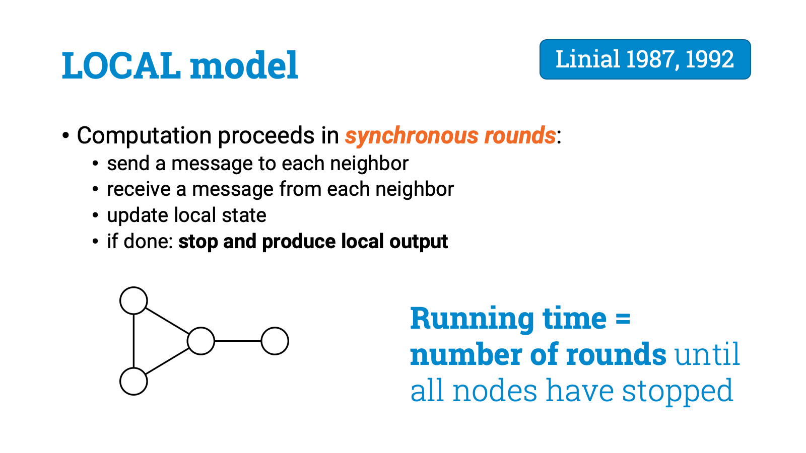
The running time is the number of rounds it takes until all nodes have stopped. So in this model time is the same thing as the number of communication steps. Good.

But there is another way to define the same thing. Let’s think about what we can do in $T$ rounds in this model. We didn’t restrict message size, we didn’t restrict local computation. So in each round everyone could tell everything they know to all of their neighbors! And this is also the best thing that you could do, you can’t tell something you don’t know, and telling less won’t help.

Let’s see what this means. Before the first round each node knows only its own identifier and its own degree and whatever local inputs it had. So basically you know only your radius-0 neighborhood. And this is all that you can tell your neighbors in round 1.

But now if everyone tells this to each neighbor, everyone will know who their neighbors are. So after 1 round, all nodes are aware of their radius-1 neighborhoods.

And in the second round everyone will tell this to all their neighbors. So everyone will learn what is the radius-1 neighborhood of each neighbor. And if you put together this information, you will have a full picture of your radius-2 neighborhood!

And you can continue this way. After round 3, everyone knows their radius-3 neighborhood.

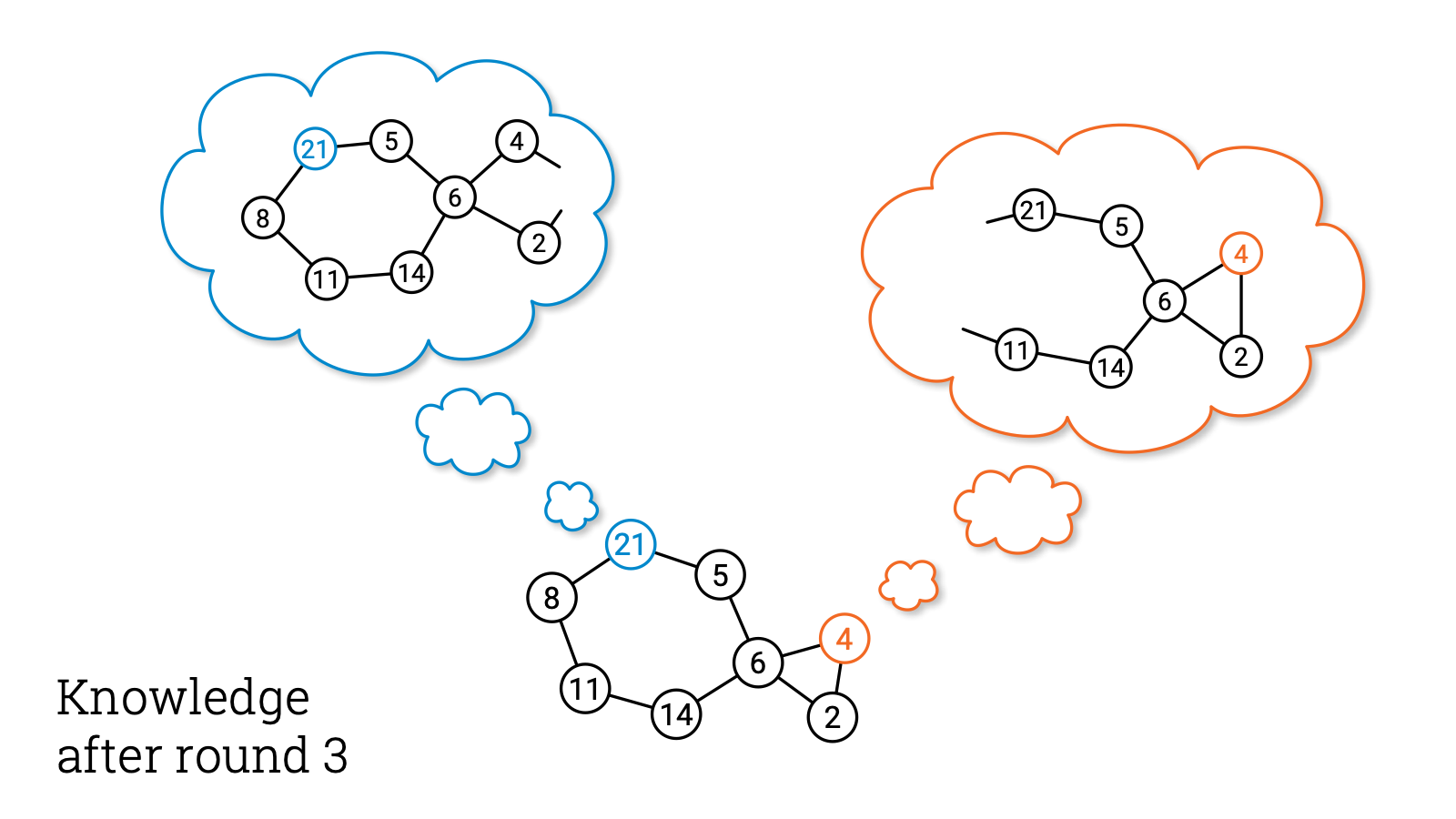
After round 4, everyone knows their radius-4 neighborhood. And so on. So at best in $T$ rounds you can learn everything up to distance $T$, and nothing more.

And if you stop after $T$ rounds and announce your local output, then whatever you output has to be a function of the information that was there in the network within distance $T$ from you. So now we have another equivalent way to define algorithms in the LOCAL model: an algorithm that runs in time $T$ is simply a mapping from radius-$T$ neighborhoods to local outputs!

This means that time and distance are interchangeable in the LOCAL model. And therefore fast distributed algorithms are also highly localized. If we have a fast algorithm, each node makes decisions based on the information that was available in its local neighborhood.

So let’s recap, all these notions are the same in the LOCAL model:

• What is the running time?
• Or, how many communication rounds are needed?
• Or, what is the locality of the problem?
• Or, how far do you need to see in the graph?

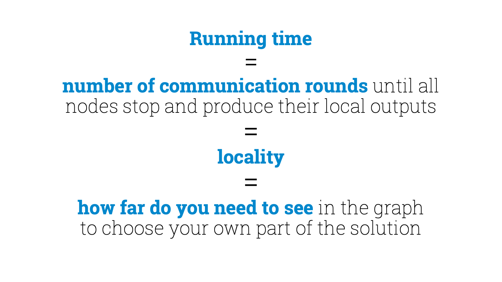
So we can rephrase our key question as follows:

• Which computational problems can be solved by using only local information?
• And which computational problems are inherently global?

Now let’s be a bit more careful and explain what we actually mean when we say something like “you can solve this problem so-and-so fast in the LOCAL model.” We’ll look at graph problems here.

Let’s take an example, let’s look at something like the task of finding a maximal independent set: We want to find an independent set of nodes, so that no two nodes are adjacent to each other. And we want it to be maximal in the sense that you can’t add any nodes to it. Now please note that this is a trivial problem from the perspective of centralized algorithms. There is a simple linear-time solution: you can just greedily pick nodes until you are stuck.

Now what does it mean if I claim I have a distributed algorithm $A$ that finds a maximal independent set in $T$ rounds in some graph family? Then this is a worst-case guarantee:

• you can take any graph from this graph family,
• you can pick any assignment of unique identifiers in the graph,
• you can run algorithm $A$,
• and it will stop in at most $T$ rounds and produce a valid solution.

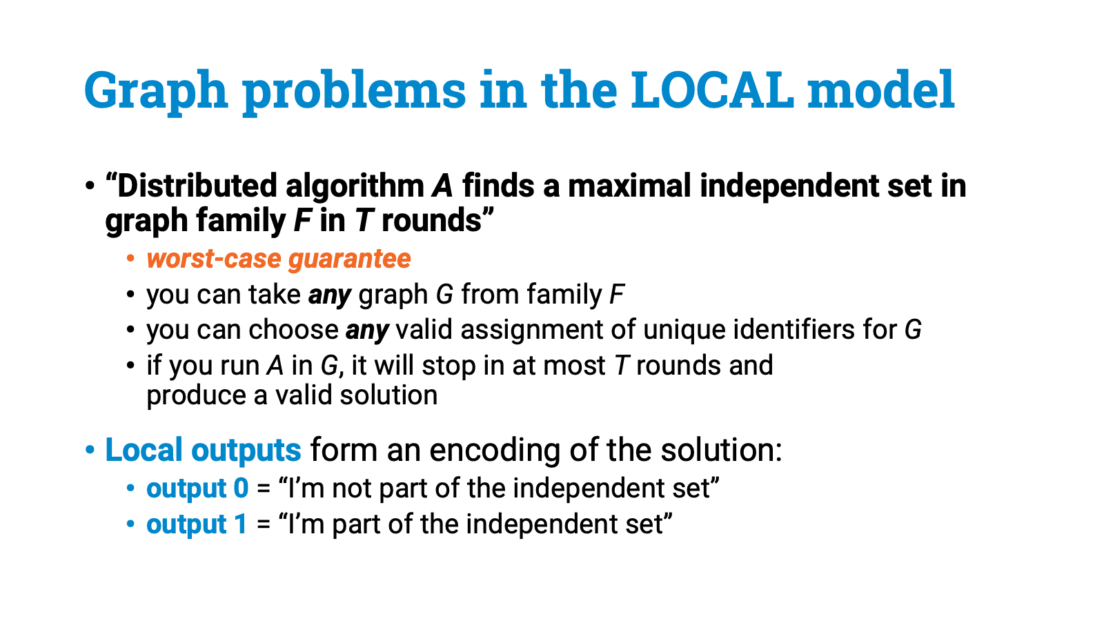
And please note that the solution is produced in a distributed manner. Each node just produces its own part of the solution. Zero or one. Whether this node is part of the independent set or not.

And if we say that the distributed complexity of some graph problem is $T$ rounds, then we just mean that the fastest possible algorithm for this problem solves it in $T$ rounds.

Of course there are few problems that can be solved in constant time, so usually $T$ is some function of $n$, which is the number of nodes. Maybe $T$ is $O(\log \log n)$ or $O(\log n)$, or $O(n)$, or something like that.

And at this point is good to note that in this setting linear time is trivial! If we have a connected graph, in a linear number of rounds all nodes can learn everything about the graph, and then the rest is just local computation. So linear time here is basically brute force. And if the complexity of some graph problem is linear, then it means that the problem is inherently global. You can’t solve it unless you see the whole graph.

And of course it isn’t that surprising that there are lots of graph problems that are global. Something as simple as coloring a path with 2 colors is an example of a global problem.

Let’s quickly prove it. Assume you had some way of solving it in sublinear time. So along a long path, these two nodes could pick their own colors based on the information in their local neighborhood only.

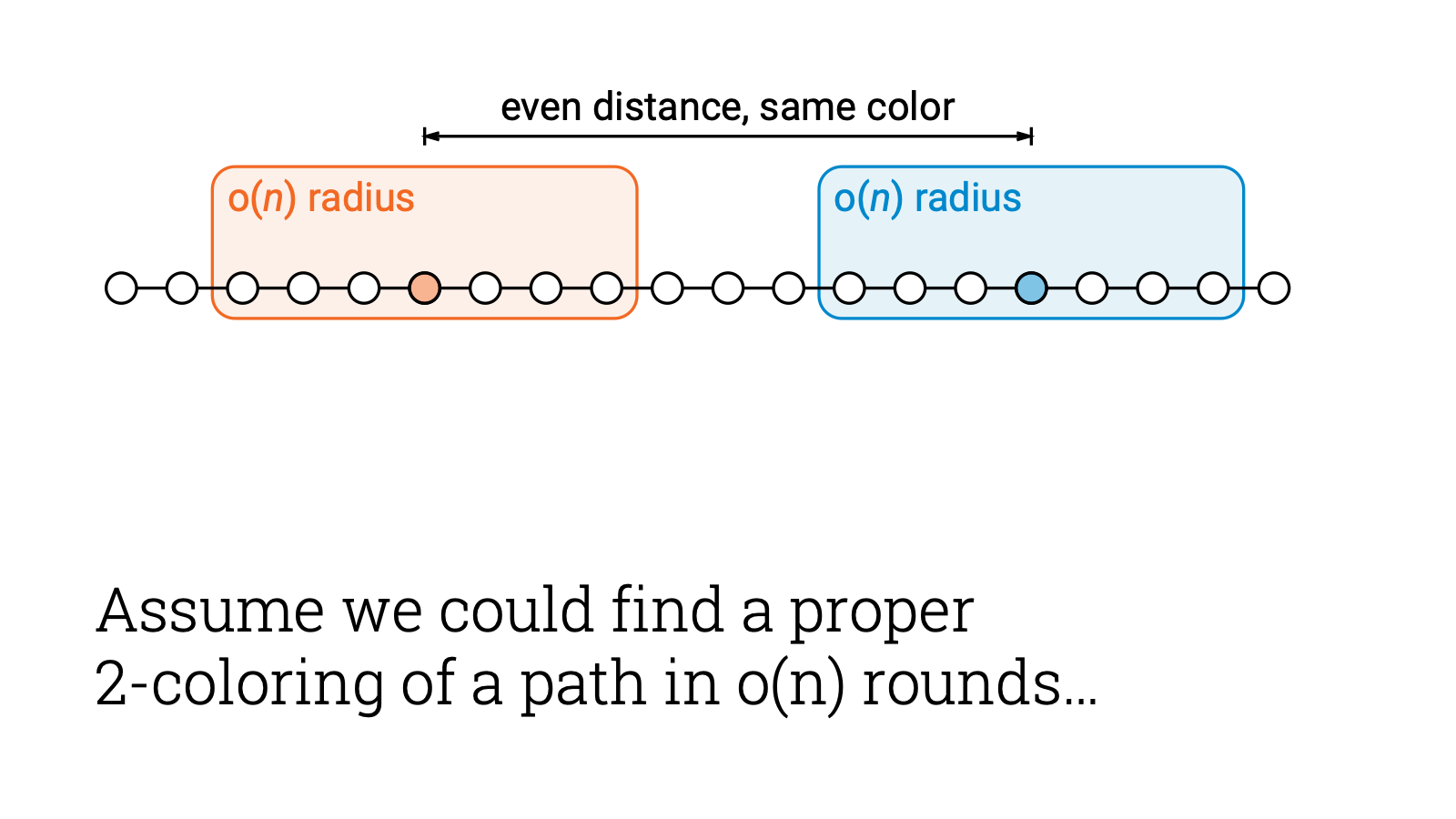
Let’s assume the distance between the nodes is even, so they pick the same color, let’s say black.

But let’s then modify the input graph like this. We just move this one node to a new place, keep everything else the same, including all unique identifiers.

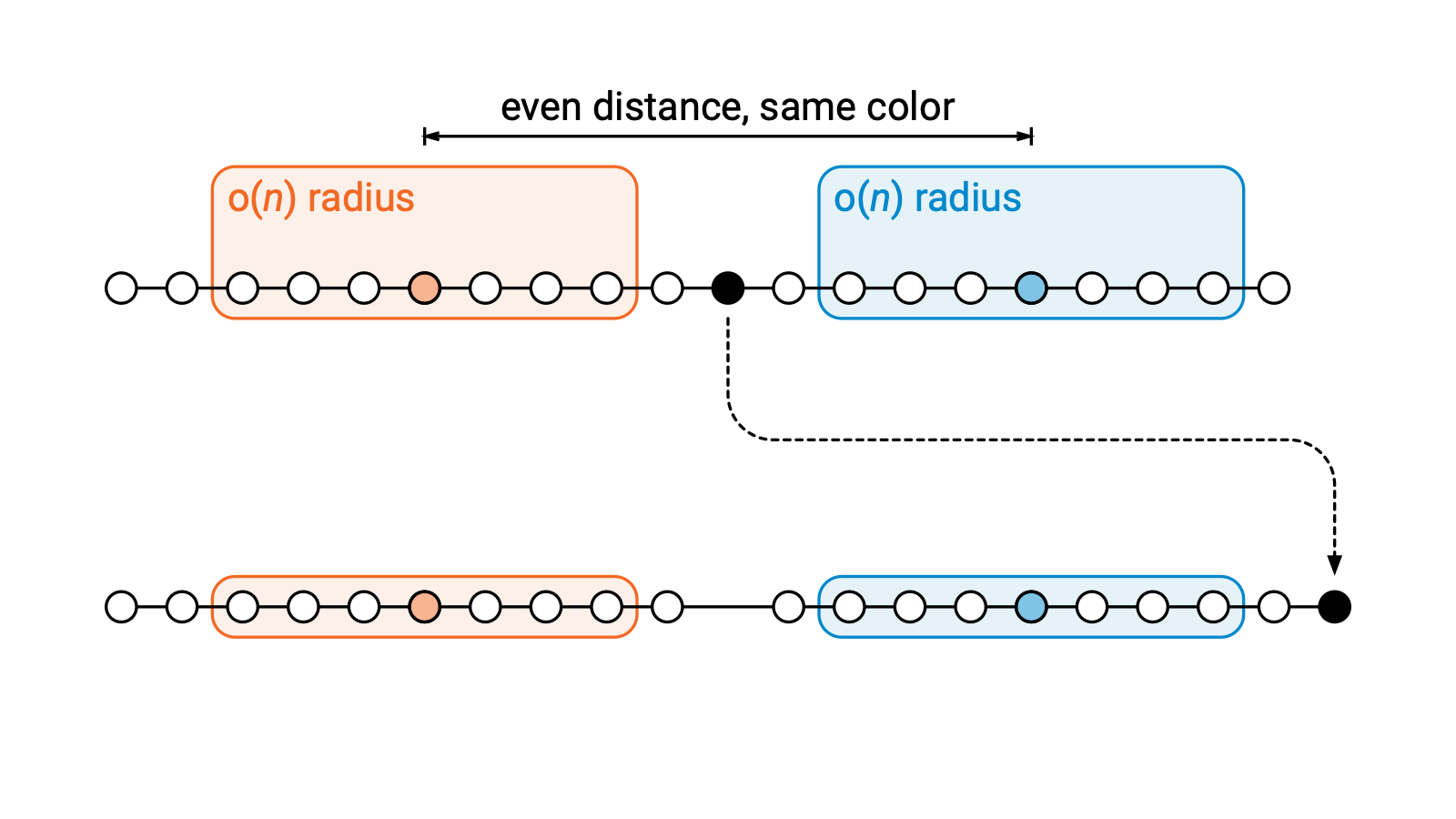
These two local neighborhoods don’t change. So the local outputs of these two nodes won’t change, either. So both nodes will still output the same color.

But the distance between the nodes is now odd, so somewhere along the path the coloring can’t be right.

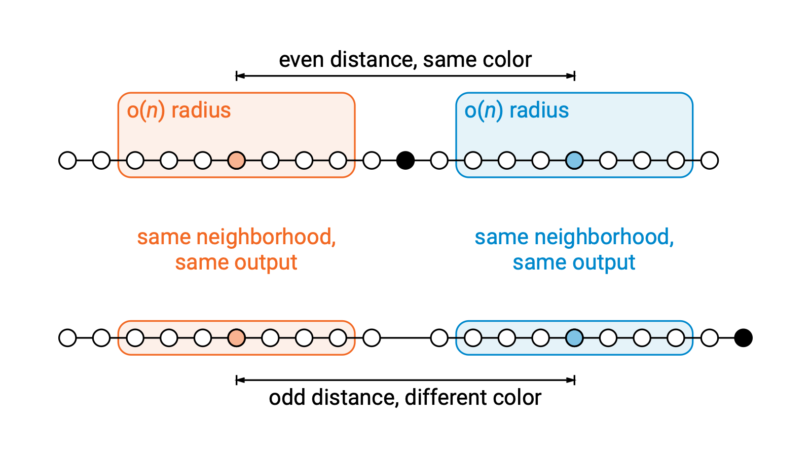
So any sublinear-time algorithm will fail. Linear-time brute force algorithms are the only possibility here.

It’s easy to give a long list of problems that are global. But what’s more surprising is that there are also lots of problems that can be solved in highly sublinear time.

For example, if we relax the problem just a bit and look at the problem of coloring a path with 3 colors, you can do much better! You can now solve this problem in $O(\log^* n)$ time!

And there is more, we can also prove that $\Omega(\log^* n)$ is the best that you can do.

So the complexity of 2-coloring paths is linear, while the complexity of 3-coloring paths is $\Theta(\log^* n)$. And it doesn’t get easier if you add more colors, 10-coloring is still $O(\log^* n)$. And randomness doesn’t help, it’s still $O(\log^* n)$ also for randomized algorithms.

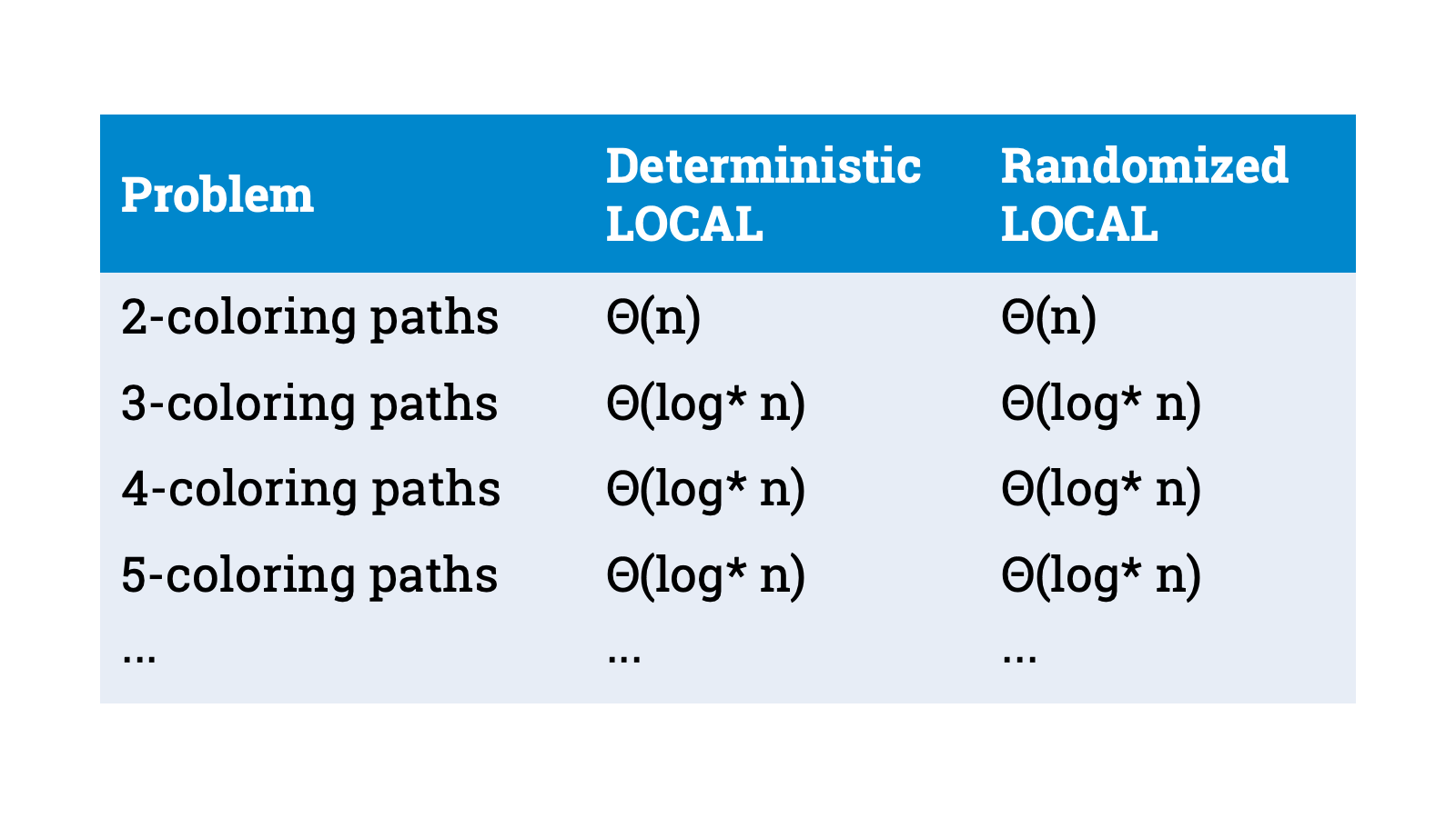
So there are many graph problems that are hard to solve in the LOCAL model, they are inherently global, you need linear time. And there are many graph problems that are easy to solve in the LOCAL model. They can be solved in highly sublinear time, for example, in $O(\log^* n)$ time.

But what’s the big picture here? What does the landscape of locality look like? The locality of graph problems has been studied actively since the 1980s, but a lot of early work focused on individual graph problems. You fix a specific problem, prove upper bounds, prove lower bounds. Or you fix a specific problem, and connect it through reductions to problems studied previously.

We got lots of individual data points, but we had no idea what the landscape really looks like. We didn’t know if these are typical, representative examples, and we didn’t learn pretty much anything that would be directly applicable to new problems.

Now all this started to change only very recently, some 5 years ago. But first we need to go back in time to the 1990s, when Naor and Stockmeyer introduced a simple but important concept: locally verifiable problems.

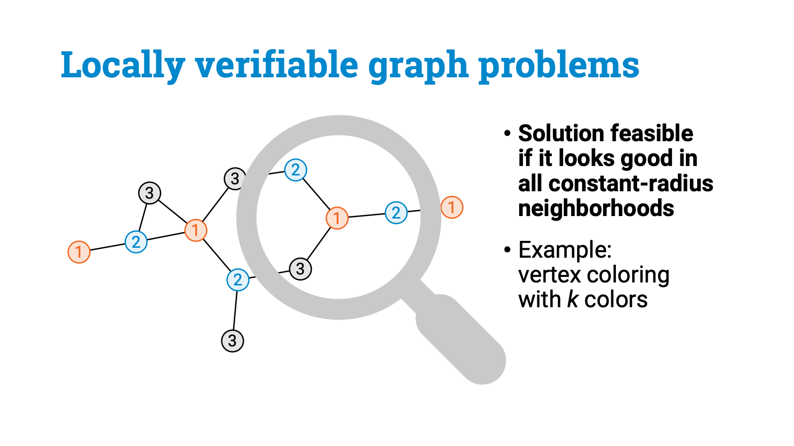
We say that a graph problem is locally verifiable if it is enough to check all constant-radius neighborhoods to ensure that a solution is feasible. Graph coloring with $k$ colors is a simple example of a locally verifiable problem. If I give you some labeling of the nodes and claim that it is a proper vertex coloring with $k$ colors, you can verify it by checking each local neighborhood, like this. Just look at each node and its immediate neighborhood. If the coloring looks good in all local neighborhoods, the solution is correct. So vertex coloring is a problem that is locally verifiable.

Of course not all problems are locally verifiable. For example, a minimum spanning tree is not locally verifiable. You can’t even verify that a set of edges is a spanning tree if you only look at local neighborhoods.

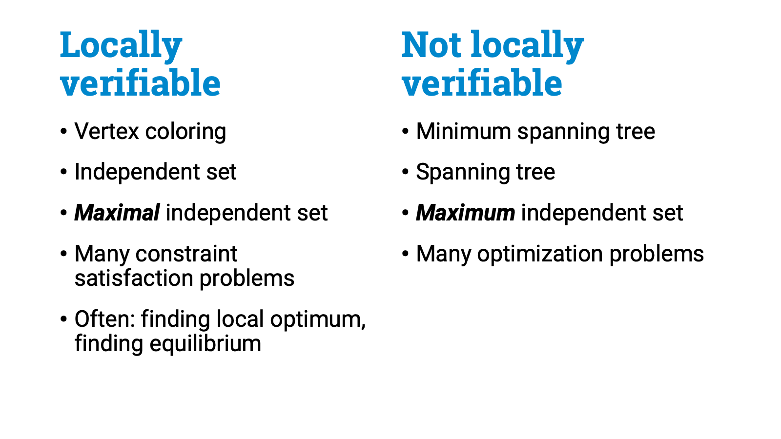
To give some further examples, an independent set is locally verifiable: it is enough to make sure a node with label 1 doesn’t have any other node with label 1 adjacent to it. And a maximal independent set is also locally verifiable: you then also check that for each 0 there is at least one node with label 1 next to it. However, a maximum independent set is something that is not locally verifiable.

Usually constraint satisfaction problems are locally verifiable. Problems in which you need to find some kind of a local optimum or a game-theoretic equilibrium are often locally verifiable. But optimization problems on the other hand are usually not locally verifiable. You get the idea.

OK, this is just a simple definition, what’s the point? Some problems are locally verifiable, some are not. Please try to bear with me a bit longer…

The first point is this. In a sense, locally verifiable problems are the distributed analogue of class NP (or, a bit more precisely, the distributed analogue of class FNP). Why do I say this? Well, if you have a locally verifiable problem, then you can solve it efficiently in the nondeterministic LOCAL model, in the following sense: each node can just nondeterministically guess its own part of the solution and then the nodes can verify the solution in constant time.

So just like the study of problems in class NP plays a big role in the classic computational complexity theory, we’d expect that the study of locally verifiable problems would play a big role in the distributed complexity theory. So is this really the case? Do we have a rich theory of locally verifiable problems? Almost there, but not quite.

It turns out that the class of all locally verifiable problems is a bit too broad to be useful. It’s hard to even imagine a nontrivial theorem that would say something useful about all locally verifiable problems. So we’ll need to narrow it down a bit to make progress. But how?

I guess nobody knew it back then, but with hindsight it turns out that Naor and Stockmeyer in their 1993 paper got it just right. They defined a family of problems they called LCLs or locally checkable labelings.

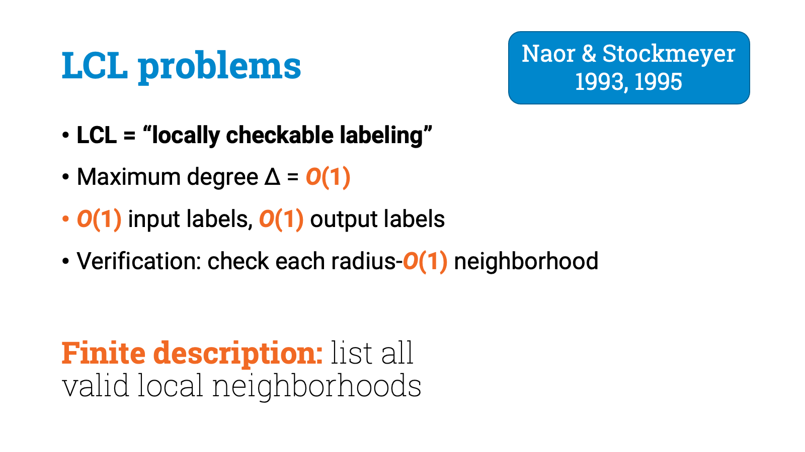
LCLs are simply the following restriction of locally verifiable problems: There is some constant maximum degree Delta, your input labels come from a constant-size set, and your output labels come from some constant-size set.

That’s it. So everything is bounded by a constant. And conveniently this means that any LCL problem has a finite description. You can simply list all feasible local neighborhoods, there are only finitely many of them.

OK, so this is once again just a definition, why should we care about this?

First, very many relevant problems that we care about turn out to be LCL problems, at least if we look at bounded-degree graphs. Vertex coloring is an LCL. Edge coloring is an LCL. Maximal matching is an LCL. Maximal independent set is an LCL. Boolean satisfiability is an LCL if you interpret it as a graph problem. And so on.

So LCLs are a broad family of problems, so if we could say something about all LCLs, it would be widely applicable.

And second, it turns out that we can do exactly that! We can prove theorems that tell something surprising and useful about the distributed complexity of any LCL problem!

But here I think the process was at least as interesting as the end result, so let’s look at the history. LCL problems were introduced in the 1990s, but what did we actually know about LCL problems back then?

We already earlier mentioned problems such as 2-coloring paths and 3-coloring paths. 2-coloring requires linear time. 3-coloring can be solved in $O(\log^* n)$ time, and it is tight. And these are clearly LCL problems, and all of this was known already in the early 1990s, thanks to the work by Cole and Vishkin, and Linial, and Naor.

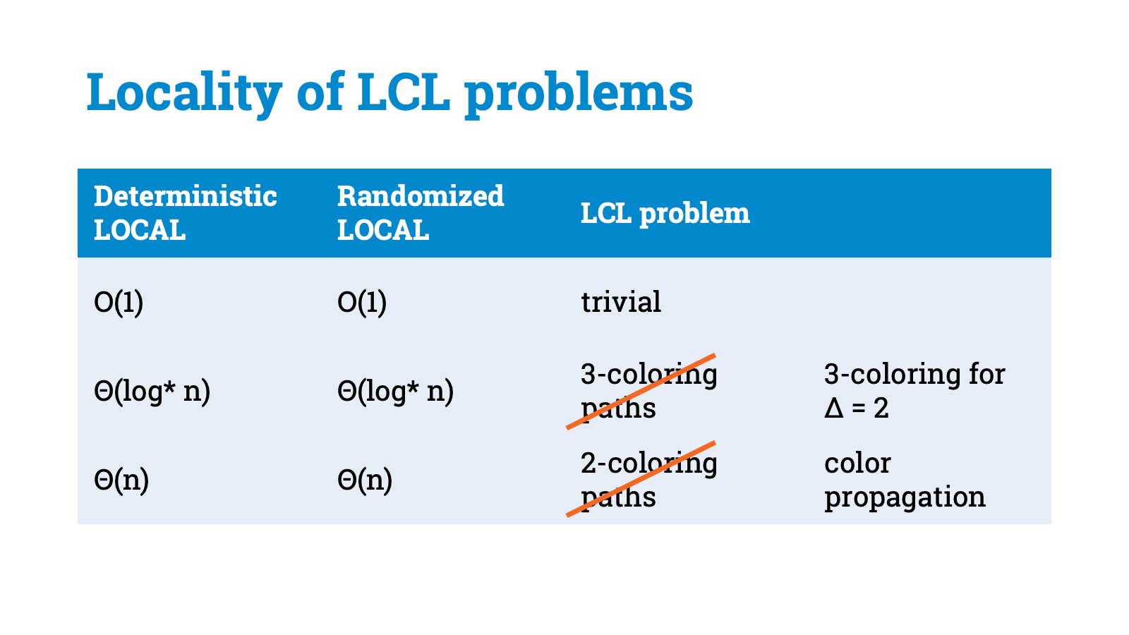
OK, OK, I cheated a bit. In these problems we had a promise that the input graph is a path, but let’s not worry about it too much, it isn’t important. You can look at the task of 3-coloring any graph of maximum degree 2, and the complexity is again $\Theta(\log^* n)$, and now it is an LCL problem in the strict sense, without any promise. And it isn’t too hard to find a global problem that is a strict LCL without any promise.

So there are LCL problems where the deterministic and randomized complexities are $\Theta(n)$. And there are LCL problems where the deterministic and randomized complexities are $\Theta(\log^* n)$. And of course there are trivial LCL problems where the deterministic and randomized complexities are constant, for example, the problem of labeling all nodes with number 1.

By the way, notice that all of these examples are problems where randomness doesn’t help at all. We’ll get back to this soon.

Let’s draw a picture. Let’s try to draw a figure that shows the landscape of all LCL problems.

I’ll put here on the horizontal axis possible deterministic complexities between local and global. These are just some examples, $O(1)$, $\Theta(\log \log^* n)$, $\Theta(\log^* n)$, $\Theta(\log \log n)$, $\Theta(\log n)$, linear. And remember that linear is as bad as it gets, linear means brute force, within linear distance you already see everything, so there’s no point looking any further.

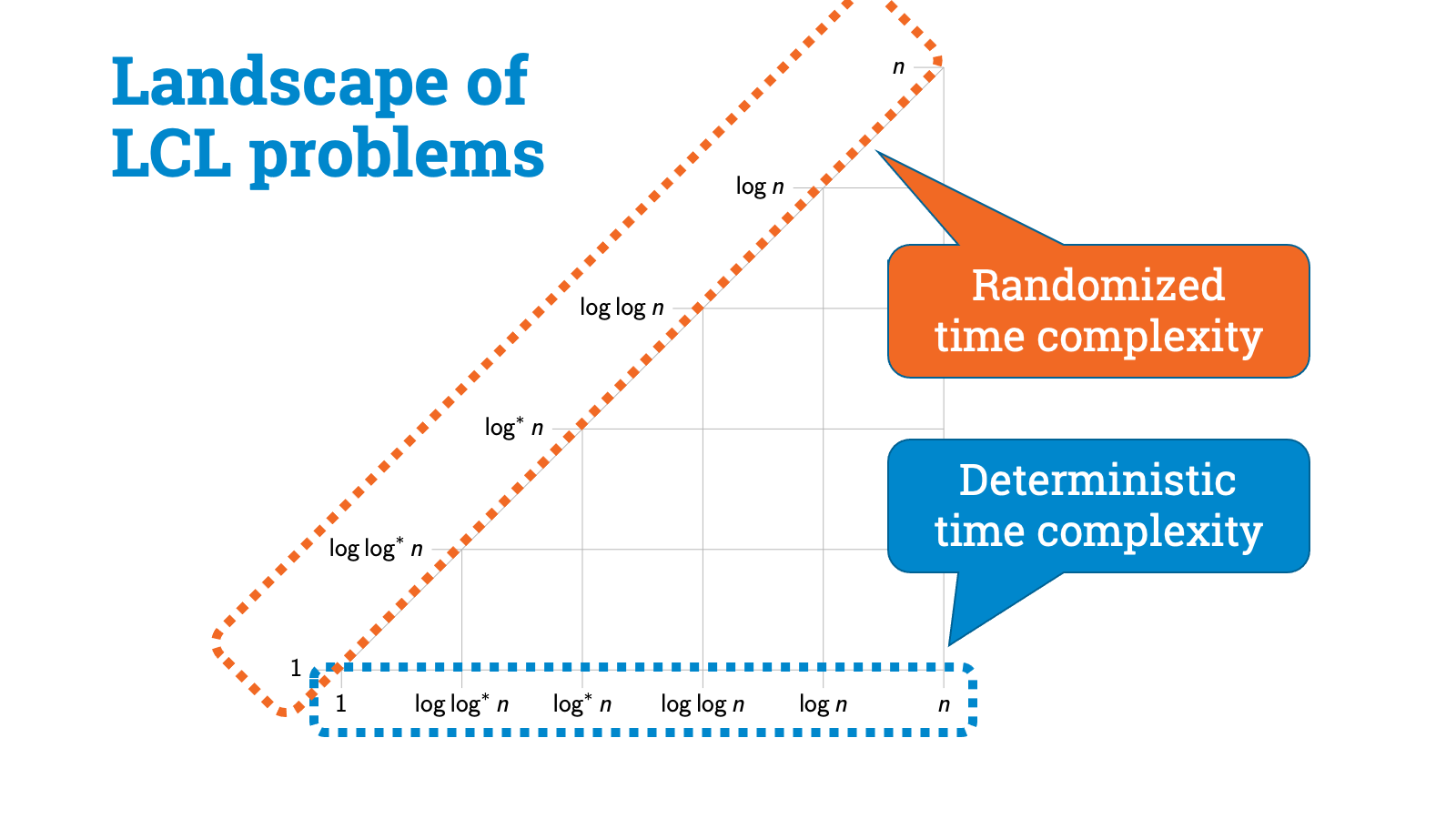
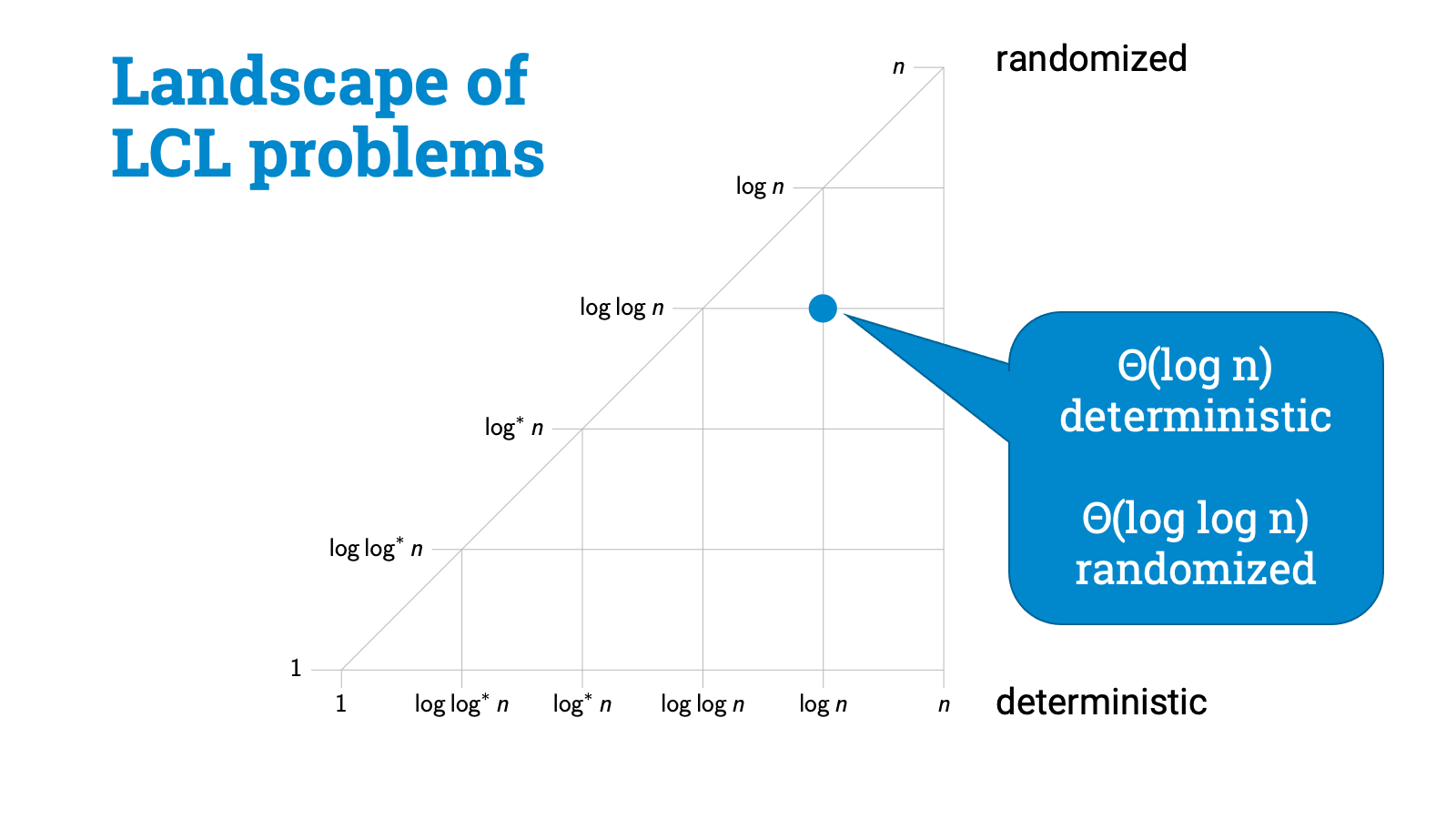
And I’ll put randomized complexities on the vertical axis. Again $O(1)$, $\Theta(\log \log^* n)$, $\Theta(\log^* n)$, and so on. Of course randomness can’t ever hurt, so we’ll be always somewhere inside this triangle.

And what I’ll try to do is to put all possible LCL problems on this map. So just to make sure all of us are on the same page, this blue dot would be some hypothetical LCL problem for which the deterministic complexity is $\Theta(\log n)$ and randomized complexity is $\Theta(\log \log n)$.

Good. So where are the dots?

As we just discussed, back in the 1990s it was already known that there are some global LCL problems that require linear time and there are some trivial LCL problems that are solvable in constant time, and then there are some curious problems that are similar to 3-coloring paths, and their complexity is $\Theta(\log^* n)$. And it turns out that this $\Theta(\log^* n)$ class is big, people have discovered tons of problems that have exactly the same complexity.

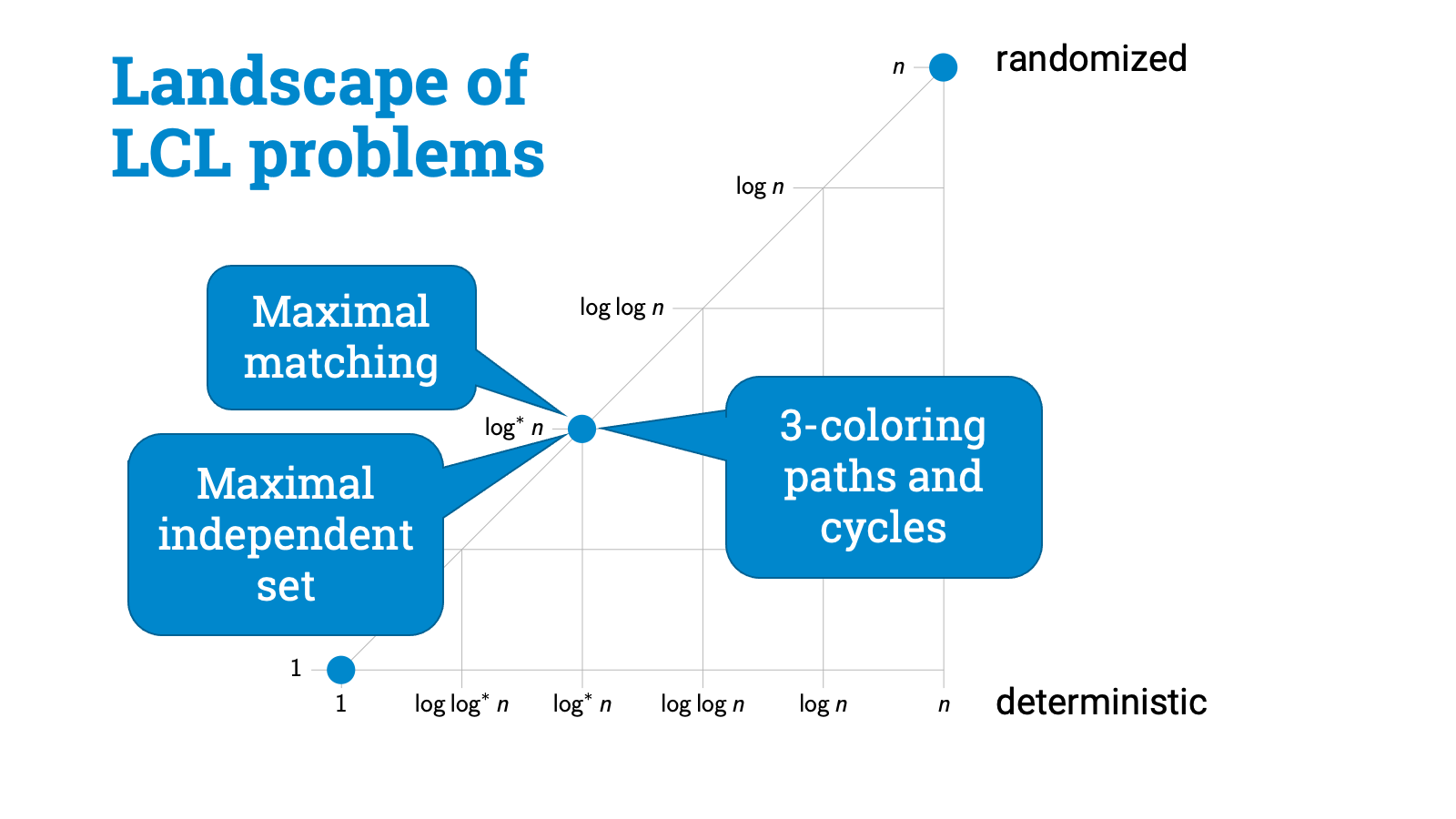
Maximal matchings — here. Maximal independent set — here. Many easy graph coloring problems — here. Basically whenever the key challenge is to break symmetry, you’ll find yourself here.

Good, so three problem classes already known in the 1990s. But what else is out there? Is this all that there is? Could we prove that all LCL problems fall in one of these classes? Or is this just the tip of the iceberg, and do we have LCL problems all over the place?

What about randomness, does it ever help? Or could it maybe help just a little bit? Or can you have problems where deterministic and randomized complexities are very far from each other?

Back then we didn’t know. And to be honest, I think people weren’t even asking these questions!

Now, fast forward some 20 years of progress and hundreds or thousands of papers related to distributed computational complexity. It’s year 2015, what do we know about LCL problems now?

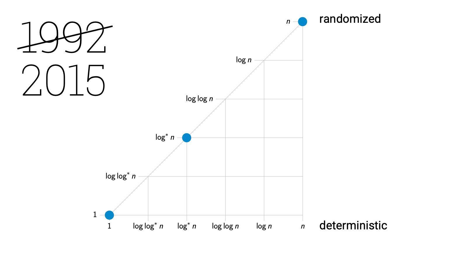
Still absolutely nothing. You may wonder why I am even talking about this if nothing is known…

But this was the key point in time, this was the moment when things started to develop rapidly. In 2016 we published a paper that showed that there is at least something else out there. We showed that there are LCL problems with intermediate complexities. Something strictly between $\Theta(\log^* n)$ and linear.

And that was the starting point. In rapid succession we got papers that proved better upper and lower bounds for the intermediate problems. For example, we got the first examples of problems in which randomness is known to help a lot.

And we got papers that introduced entirely new kinds of problems. There were infinite families of problems, with distinct time complexities. So LCL problems really come in many different shapes.

So we seem to be getting more and more LCL problems with different complexities. Not too surprising, after all, as I said earlier, this is a large family of problems.

But in parallel with these positive results, what we started to see is negative results. There were gap theorems that ruled out the existence of LCL problems in these regions. And these. And these. And finally, most recently, also these.

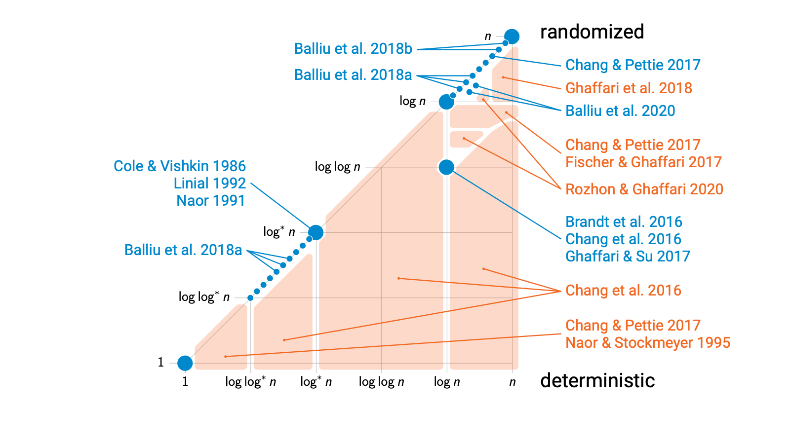
All of these orange regions are gap theorems. And if you put all these results together, a near-complete picture of the landscape of LCL problems emerges!

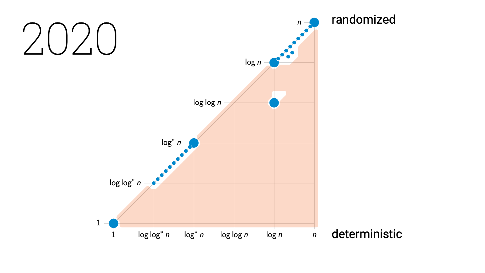
There are some tiny regions of uncharted white slices here and there, but we are now very close to a complete picture of what are possible deterministic and randomized complexities of LCL problems.

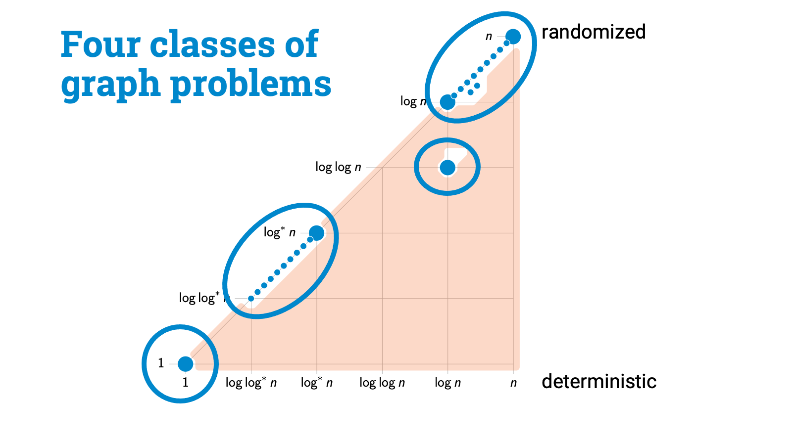
So what we see is that we have got four distinct classes of problems, and there are wide gaps between these classes. And gaps are very important, because these have got direct use both in algorithm design and in complexity theory!

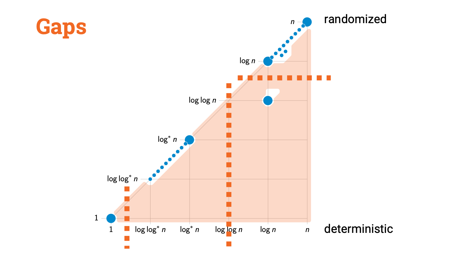
For example, assume that you have managed to design an algorithm that solves some LCL problem in $o(\log n)$ rounds with a deterministic algorithm. But we had a gap result that shows that the deterministic complexity is either at least $\Omega(\log n)$ or at most $O(\log^* n)$. So if we just touch this algorithm with the gap theorem, magic happens and we can speed it up to $O(\log^* n)$. And by the way, these gap results are not just existential, they are constructive, so we really get the faster algorithm this way.

And let’s look at another example. You are studying some LCL problem and you managed to prove that it can’t be solved in $O(\log^* n)$ time. Then just apply the gap result and you have got immediately an $\Omega(\log n)$ lower bound for deterministic algorithms and an $\Omega(\log \log n)$ lower bound for randomized algorithms!

And these applications aren’t just made-up examples. Even though these are recent results, we have already seen over and over again that we can make effective use of gap results when we do algorithm design and when we prove lower bounds.

So let’s recap now. We started with any graph problem that is locally checkable. So all that we know is that local information is enough to verify the solution. Then we asked how far you need to see to find a solution. And this picture emerges. I seriously wasn’t expecting anything like this, but of course with perfect hindsight everything makes sense. We have got here four distinct classes of problems, each with a very distinct flavor.

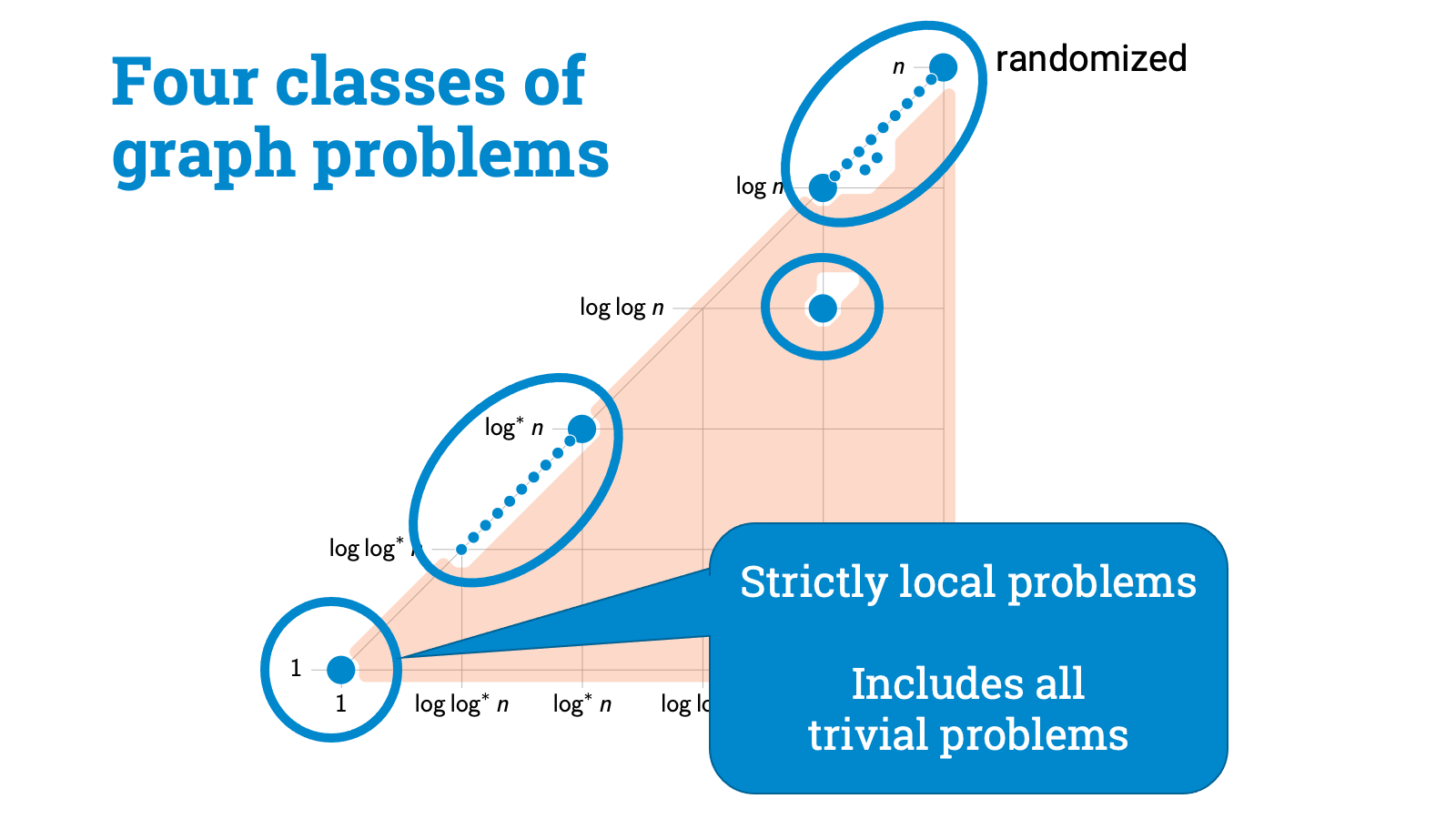
There are strictly local problems, for example, problems in which you can label all nodes with the same label.

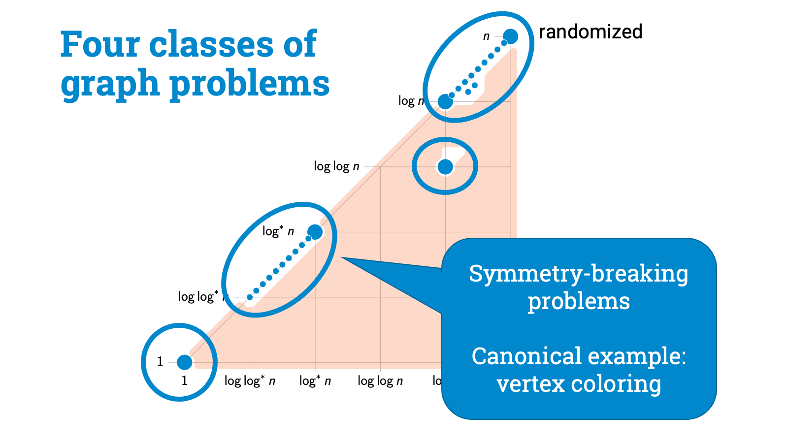
Then there are symmetry-breaking problems. Here the key challenge is that nodes need to be able to pick output labels that don’t conflict with the choices of their neighbors. Graph coloring is a canonical example of such a problem. And it turns out that graph coloring is also, in a sense, a complete problem for this class.

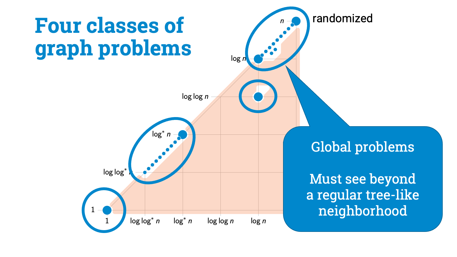
Then we have got a broad class of hard problems here. My intuition is that these problems are all global in some sense. If you are sitting in the middle of a regular tree-like neighborhood, you can’t do anything until you see something else. A leaf node. A cycle that closes. Some kind of irregularity. Here randomness may help a bit but not much.

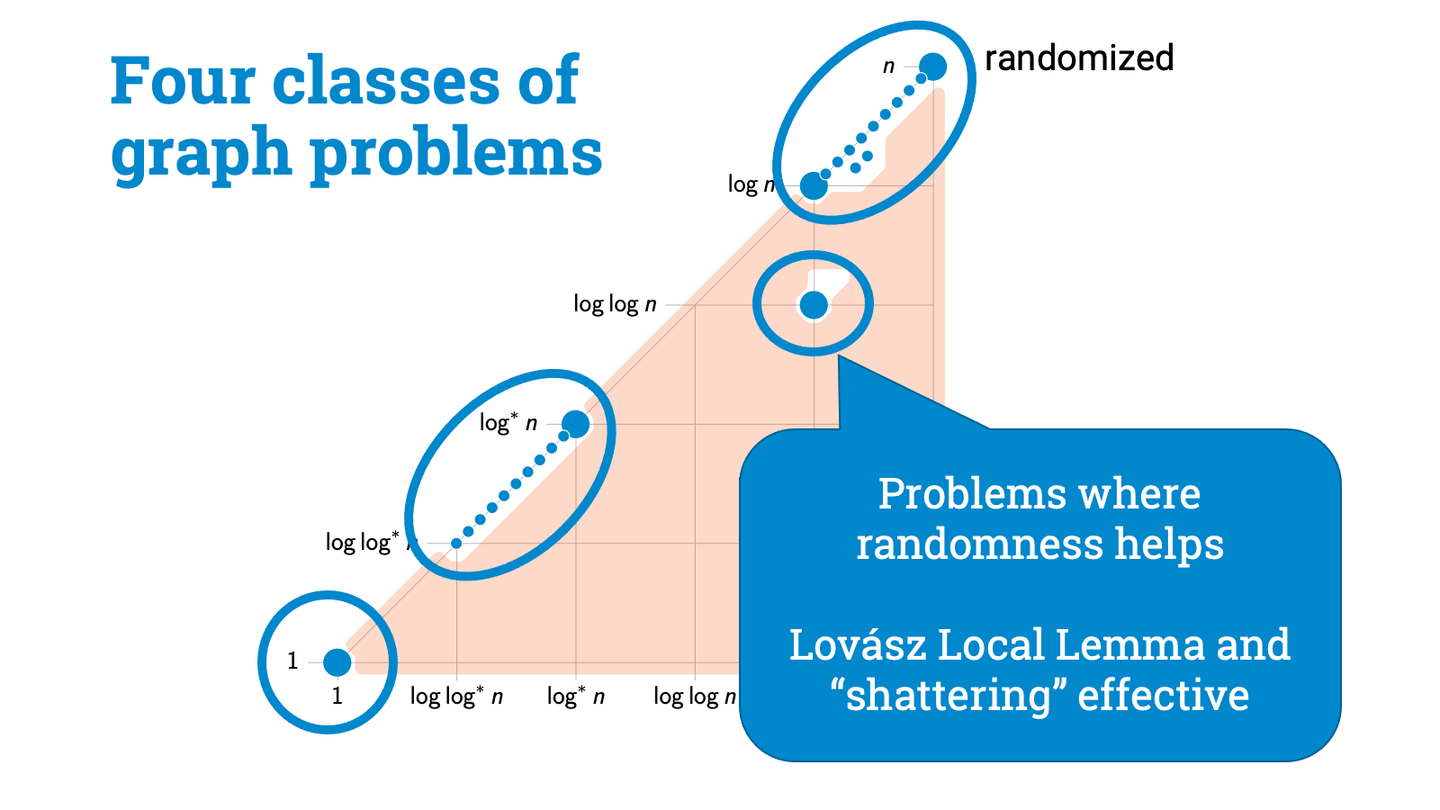
And finally, there is a very important class of problems here. This is the only class of problems where randomness helps a lot, these are problems where the deterministic complexity is something like $\Theta(\log n)$, but randomized complexity is exponentially better, only $\Theta(\log \log n)$.

Let me try to say something more about this class. In some sense, this is the class where algorithmic Lovász Local Lemma works. And this is the class where the so-called shattering technique works. But perhaps the best way to get a better feeling of this class is to show an example.

Here is a graph problem called sinkless orientation. The task is simple: you need to orient the edges so that all high-degree nodes have at least one outgoing edge. More precisely, if the degree of a node is at least 3, then its outdegree has to be at least 1.

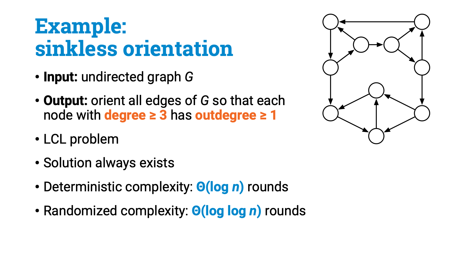
So high-degree nodes can’t be sink nodes. This is clearly an LCL problem. And if you haven’t seen this problem before, it’s a nice quick puzzle to convince yourself that this problem is always solvable. But how hard is it to find a solution in the LOCAL model?

If you are looking for a deterministic solution, then the complexity is exactly $\Theta(\log n)$, there is a matching upper and lower bound. But randomized solutions can do much better: it turns out that you can find a solution in $\Theta(\log \log n)$ rounds with high probability!

This seemingly innocent toy problem is a canonical example of a problem in this class in which randomness helps. This problem has played a key role in the development of our understanding of distributed computational complexity. Sinkless orientation was the first example of an intermediate problem that started the whole business, and it has served as a running example both in the development of algorithm design techniques and lower bound techniques. I'll come back to this problem soon.

So now we know that any LCL problem belongs to one of these four classes. But if you are given an LCL problem, can you decide what is its class? Can you write a computer program that figures out the complexity of any given LCL problem?

The really nice thing about LCL problems is that any such problem has got a simple, finite description. So you can easily write down the description of an LCL problem as a string and feed it to a computer. So at least the question is meaningful.

Could we maybe automate all of our work and write a program that automatically synthesizes optimal distributed algorithms for a given LCL problem? It probably doesn’t come as a surprise that such questions are undecidable in general. But, this certainly doesn’t mean it makes no sense to try to do it!

One of the key discoveries from the recent years is a proof technique that is nowadays known as “round elimination”. This is something completely mechanical and you can apply it to basically any LCL problem.

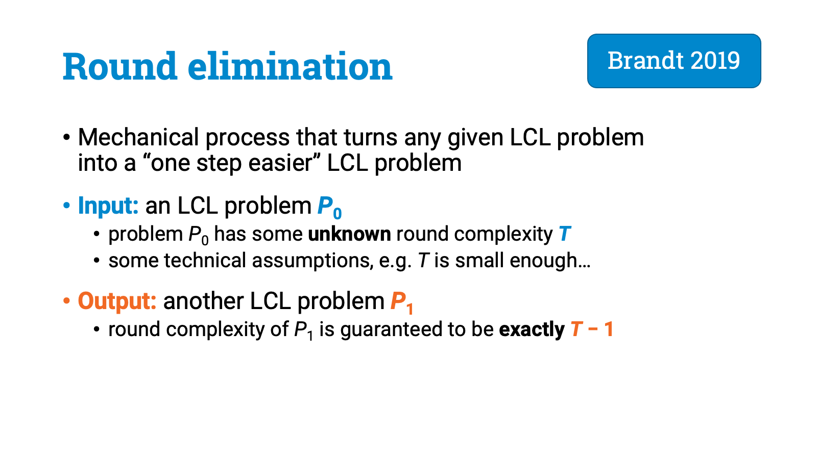
So what does round elimination do. You start with an LCL problem $P_0$ that has some unknown distributed complexity $T$, where $T$ is something small enough. You apply round elimination, and it automatically gives you some other LCL problem $P_1$ that will have complexity exactly $T-1$. You don’t need to know $T$, whatever $T$ was, you know that the complexity of $P_1$ is going to be $T-1$.

So what’s the point of all this? Well, let me give just one example.

If you have an LCL problem $P_0$ that you think might be solvable in constant time, you can just repeatedly use round elimination until you arrive at a trivial problem that can be solved in 0 rounds. If it took for example 5 steps until you got a problem $P_5$ that is solvable in 0 rounds, then you know that the complexity of the original problem has to be exactly 5 rounds. And you can even work backwards to recover an optimal algorithm that soles $P_0$ in this time.

And what’s best is that all of this is automatic, there’s nowadays a freely available open source program that does all that for you. There’s even a web interface where you can just type in an LCL problem and try your luck.

So this is something you can do with constant-time solvable problems. But what happens if you try to feed in our favorite canonical problem, sinkless orientation?

It turns out that sinkless orientation is a fixed point for round elimination. So you start with a problem that has complexity $T$, and get back the same problem, which should have now complexity $T-1$.

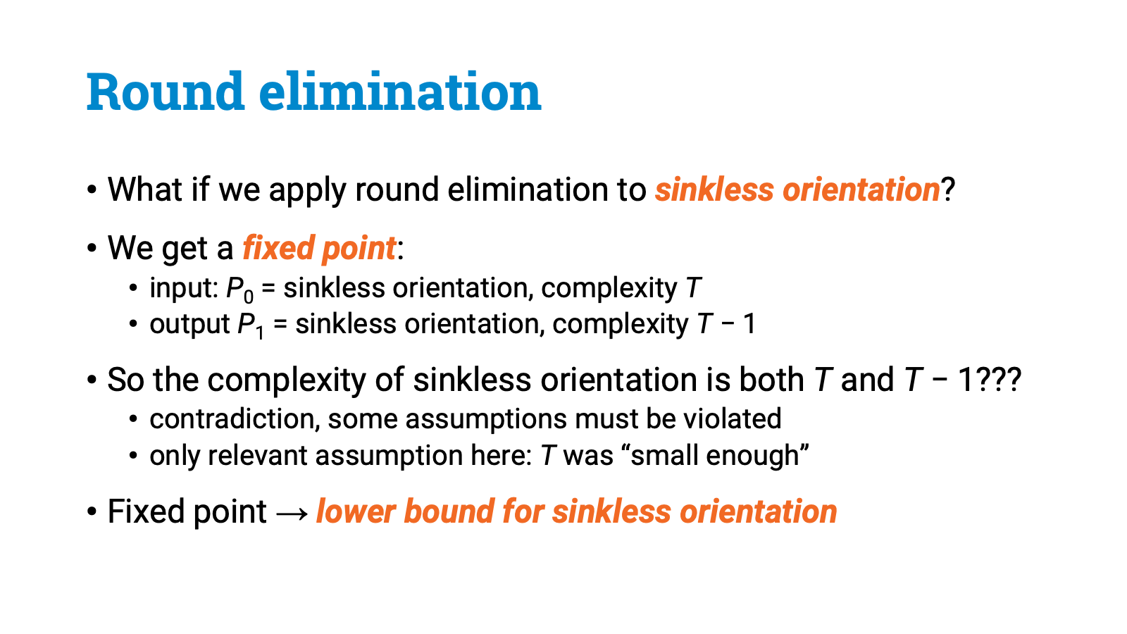
Of course this doesn’t make any sense, so the original problem has to violate one of the assumptions. And basically the only assumption that we had is that $T$ is small enough. So whenever you have a nontrivial problem that is a fixed point for round elimination, you automatically get a lower bound. You enter a problem to the round eliminator tool, see that it is a fixed point, and you can immediately conclude that the problem requires at least $\Omega(\log n)$ rounds with deterministic algorithms and at least $\Omega(\log \log n)$ rounds with randomized algorithms.

And the punchline is this: In our STOC 2016 paper we spent several pages of careful analysis to prove a lower bound for the sinkless orientation problem. Today I can open a web browser and get the same result with a couple of mouse clicks.

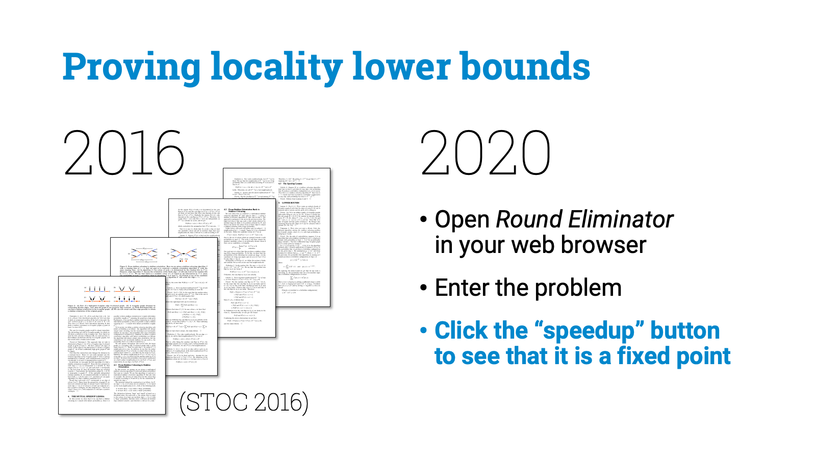
And not just for sinkless orientations, but for all LCL problems that happen to be fixed points in round elimination. We don’t know yet which problems are fixed points, but we are discovering more all the time.

Let’s recap. In this talk I have tried to give you some idea of the rapid progress that we have had in the recent years in our understanding of the distributed computational complexity.

I focused here on the LOCAL model, which is particularly elegant: time equals distance, fast algorithms are also highly localized algorithms.

And I focused on one important family of graph problems: we looked at LCL problems, where solutions are easy to verify in a distributed setting, and we asked how easy it is to find a solution.

And one of the big discoveries of the recent years was this classification of all LCL problems. We have got four broad classes. There are wide gaps between the classes. And there is tons of interesting fine-grained structure.

And as we briefly discussed, we have got also automatic techniques that can help us to both discover algorithms and prove lower bounds for many LCL problems.

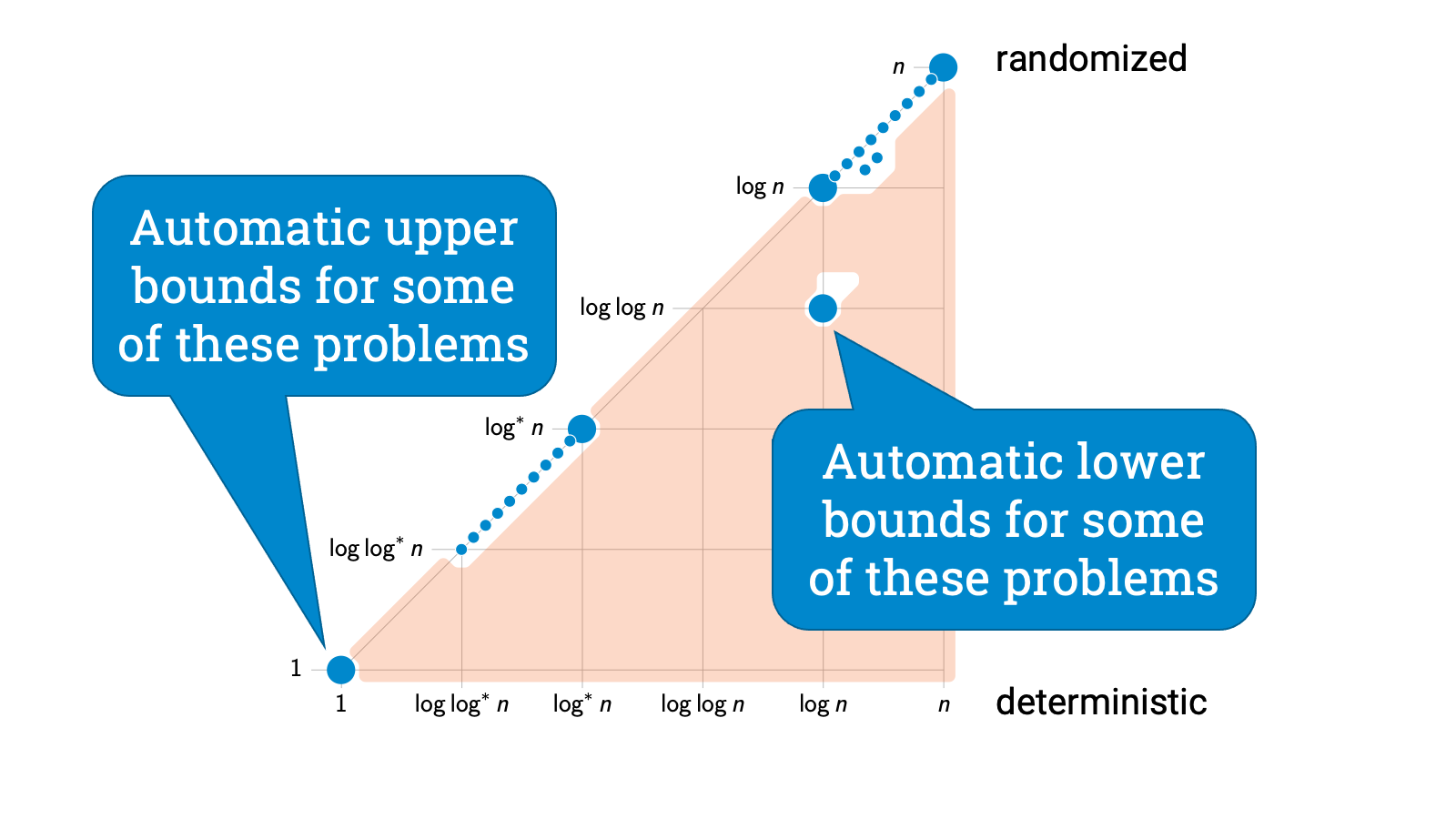
Now of course this is not the end of this line of research, but only the beginning. The key open questions are these:

• First, what happens when we step outside the class of LCL problems?
• Second, what happens when we look at other models of computing besides the LOCAL model?

Can we take all the recent discoveries that we have discussed today and transfer them to new settings? Can we completely classify more than just LCL problems? Can we develop automatic proof techniques similar to round elimination for other models of computing?

Nobody knows yet, but the research community is actively working on these questions. I hope you enjoyed this brief overview of what computational complexity nowadays looks like to someone working in distributed graph algorithms. Many thanks for watching, and if you want to know more, please feel free to ask me!